Excel functions & formulas
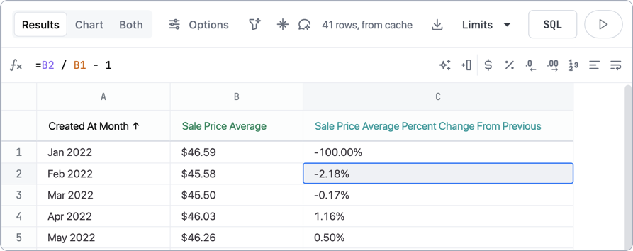
Table calculations create ad-hoc metrics that are performed post query processing on the result set à la Excel or Sheets. They can build contextual metrics like percent of row or column, period over period changes, or other calculations to customize analyses or visualizations.
Excel functions can be used to create formulas that manipulate data and calculate strings and numbers. Omni's list of available functions in each category can be found below.
Preset quick-add functions
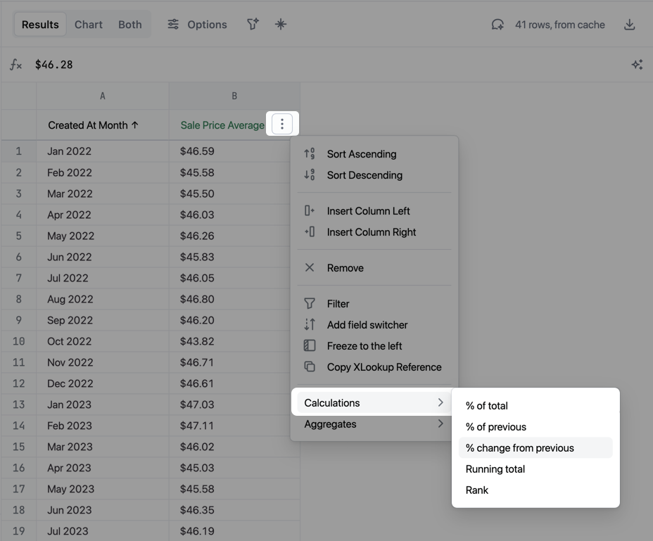
Several functions are available as quick calculations on top of numerics in the result set. Quick calculations are only available on UI-generated result sets or 'SQL Super Powers' result sets. Quick calculations are also available across pivots when active (for example, row running total).
- % of total, % of total (row)
- % of previous, % of previous (row)
- % change from previous, % change from previous (row)
- running total, running total (row)
- rank, rank (row)
How to...
Calculate with excel functions
- In a workbook, navigate to the "Add a column" icon or select the three dot menu that appears on the right-hand side of a column header. Note: In order to perform a caculation, be sure that the fields (dimensions or measures) being referenced in the table calculation are selected in the workbook query.
- Start a new calculation from the function editor or directly in the cell. The calculation must start with an
=
sign. All alphabetic characters must be wrapped in double quotes, e.g."Hello world"
, unless the text is referring to a specific cell or column. Single quotes are not valid strings in Omni (or Excel/Sheets).
Promote table calculations to the model
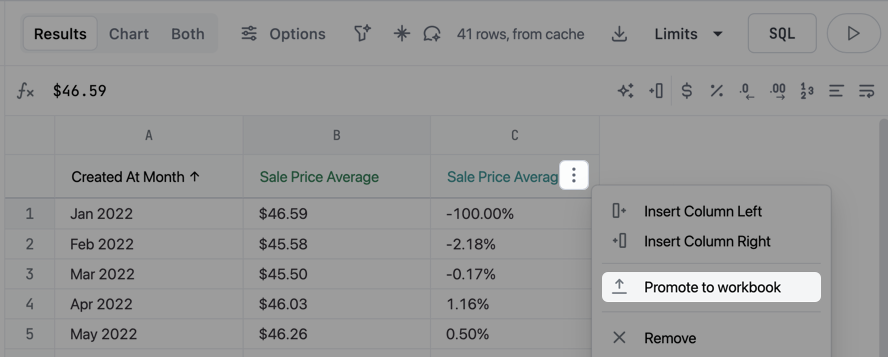
Calculations can be promoted to dimensions or measures for reuse into the workbook, then optionally into the shared model. Depending on the type of calculation some limitations will exist, i.e. calculations based on other calculations, calculations that include a range reference.
Calculate with preset quick-add functions
- In a workbook, select the three dot menu that appears on the right-hand side of the column header. Towards the bottom of the dropdown menu there are preset Calculations readily available to use with existing workbook results.
- Alternatively, the same Calculations mentioned in the previous step are available as quick icons from the function editor.
Calculate with AI
Calculations AI allows users to create table calculations with natural language inputs.
Metadata sharing
- NO DATASET RESULTS ARE PASSED TO CHATGPT.
- Omni only passes through the column IDs and how they map to a table i.e.
{A: users.id, B:user.state, C:order.count}
to Calculations AI. - If you would like to disable this feature, please email Omni at support@omni.co
How to use calculations AI
- In a workbook, navigate to the "Add a column" icon or select the three dot menu that appears on the right-hand side of a column header. Note: In order to perform a caculation, be sure that the fields (dimensions or measures) being referenced in the table calculation are selected in the workbook query.
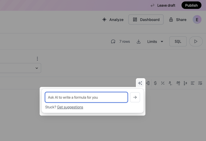
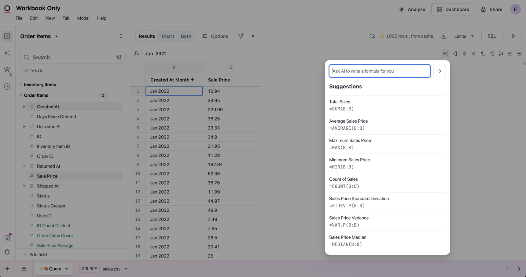
- Under the new table calculation column, select the initial cell to start formula and then select the "Natural Langugage Formula".
- When prompted, add the desired formula in plain text. e.g.
Multiply 'Order Total' with 'Order Count'
Add free-text values
- In a workbook, navigate to the "Add a column" icon or select the three dot menu that appears on the right-hand side of a column header. Note: In order to perform a caculation, be sure that the fields (dimensions or measures) being referenced in the table calculation are selected in the workbook query.
- Under the new calculation column, add free-text values in the desired cells.
- 💥
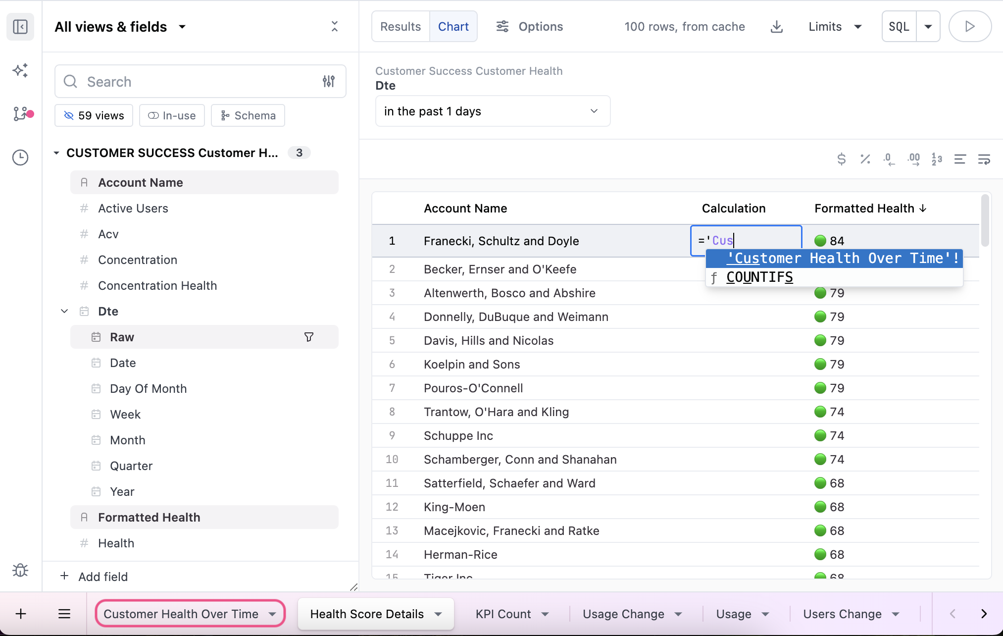
One way to leverage the free-text values is to cross-reference columns or cells across other tabs. Create a new column and then enter an equal sign and ` to pull up the tab names in the cell.
Excel-style functions
Calculation building blocks
Calculations consist of a handful of “primitive” types, which can be thought of as the compositional building-blocks of calculations.
String Literals
String literals are just strings, you might use string literals as arguments in a concatenation function.
example: "Hello Omni"
notes:
- String literals must be wrapped in double quotes.
Number Literals
Number literals are just numbers.
example: 123
notes: - They can be used as function arguments or alone.
Logical Literals
These are boolean values (true or false) values.
example: TRUE
or FALSE
notes:
- They must be all caps to be valid otherwise they’ll be interpreted as a field reference.
Unary Operators / Negation
Negates a variable value.
syntax:: -value
example: -orders_sum
- returns the negative value of the daily budget
notes:
- Unary operators in a broad sense are operators with only a right operand.
- In this example, the negative unary operator is used to express negation, such as “-1”.
- The “+” operator can also be used as a unary, however we ignore it for the most part since “+1” and “1” are logically equivalent.
Cell Reference
A cell reference is a grid notation pointing to a specific cell in a data set.
example: C2
notes:
- For example,
C2
references the third column “C” and the second “2”. - The row can be omitted to reference the column. The column can also be referenced by name (ex: users.count)
- Omni handles cell references by typically being in reference to the first row of data, and your calculation will be copied down to all following rows with the number changed to offset how many rows down you are.
- For example, the calculation
C1 + 10
will apply on the first row, but the second row will executeC2 + 10
, the third rowC3 + 10
and so on.
Cell Range Reference
A compound cell reference that describes a span between one cell and another. Cell ranges are essentially arrays of data representing a subset of a given column.
example: C1:C5
notes:
- Cell ranges are inclusive, so
C1:C5
will include the following cells [C1,C2,C3,C4,C5]
Supported functions
Functions are predefined formulas designed to make calculations on values easier.
examples:
SUM(1,2,3)
NOW()
notes:
- They accept “arguments” which are typically one of the other kinds of primitives, for example
SUM(A1,B1,100)
has two cell references and a number as its arguments. - We aim to be compatible with Excel or Sheets wherever possible. So, oftentimes, those docs are good for fleshing out your understanding of our functions. We have a few differences which will be noted below.
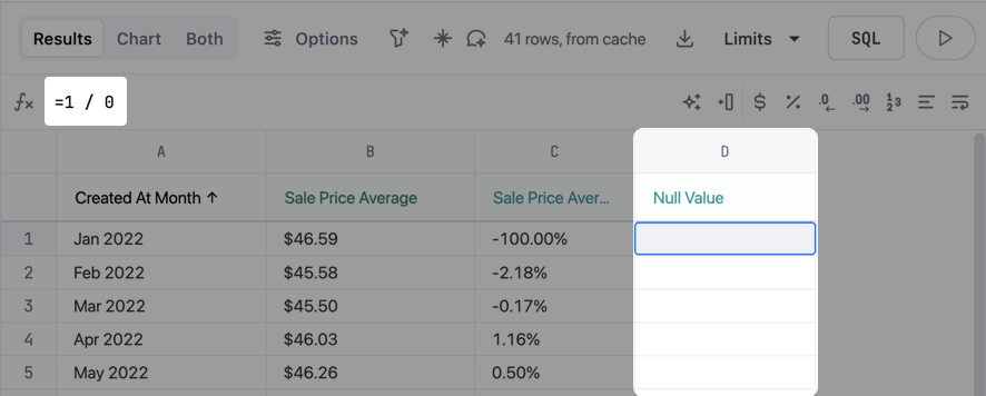
- To return a
null
value, use1/0
Math functions
Binary Operators / Math
Binary operators are operators that take both a left and right operand.
example: value1 + value2
notes:
- Expressions follow the standard order of operations. That is, the expression multiplies and divides before it adds and subtracts. You can use parentheses to clarify the expression or alter the order.
- In the case of
1 + 2
, “1” is the left operand, “+” is the binary operator and “2” is the right operand.
Supported binary operators:
- concat:
&
- plus:
+
- minus:
-
- multiply:
*
- divide:
/
- exponentiate:
^
- inequalities:
<
,<=
,=
,>
,>=
ABS
Returns the absolute value of a number.
syntax: ABS(x)
- x is any numeric type field or value
example: ABS(-14)
notes:
- For more examples, see Google Sheets ABS() function documentation.
AVERAGE
Averages a list of numbers.
syntax: AVERAGE(list)
- x is the list of numbers that can be composed of number literals (10), cell references (A1), cell ranges (B4:B9), and column references (C:C).
example: AVERAGE(1, 2, 3, 4)
notes:
- Omni will apply the average function to all values in that column.
- For more details, refer to the Google Sheets AVERAGE() function documentation.
CEILING
Round numbers up.
syntax: CEILING(x, <significance-optional>)
example: CEILING(A1, .05)
notes:
- This optionally accepts a second argument to convey significance.
- More information can be found in the Google Sheets CEILING() function documentation.
CORREL
Returns the correlation coefficient of the array1 and array2 cell ranges.
syntax: CORREL(array1, array2)
example: CORREL(A1:A3, B1:B3)
notes:
- More information can be found in the Google Sheets CORREL() function documentation.
COUNT
Counts the number of cells that contain values in the column.
syntax: COUNT(x)
- x is the cell references (E1), cell ranges (B4:B9), or column references (C:C).
example: COUNT(A1)
notes:
- The count applies to the entire column. The count does not start from the specified cell.
- For additional details, see the Google Sheets COUNT() function documentation.
COUNTA
Counts the number of cells that are not empty.
syntax: COUNTA(x)
- x is the cell references (E1), cell ranges (B4:B9), or column references (C:C).
example: COUNTA(A1)
COUNTIF
Counts the number of cells that contain values that meet a given criteria.
syntax: COUNTIF(cell_range, criteria)
- cell_range – the range the criteria_argument is applied to
- criteria – the test applied to the specified cell range
example: COUNTIF(A2:A5, A1 >= 2)
notes:
- COUNTIF() is not case sensitive.
- Omni does not yet support criteria of type string.
- Refer to the Google Sheets COUNTIF() function documentation for more details.
COUNTIFS
Counts the number of cells that contain values that meet given criteria; this function supports multiple criteria arguments.
syntax: COUNTIF(cell_range, criteria1, [criteria2-optional])
- cell_range – the range the criteria is applied to
- criteria – the test criteria applied to the specified cell range
example: COUNTIFS(A1:A5, A1 > 2, B3:B10, B1 > A1)
notes:
- COUNTIF() can only perform conditional counts with a single criterion. To use multiple criteria, use COUNTIFS().
- COUNTIFS() is not case sensitive.
- Omni does not support string criteria.
- More information can be found in the Google Sheets COUNTIFS() function documentation.
COVAR
Returns covariance, the average of the products of deviations. Equivalent to COVAR.S.
syntax: COVAR(array1, array2)
example: COVAR(A1:A10, B1:B10)
notes:
- More information can be found in the Google Sheets COVAR() function documentation.
COVARIANCE.P
Returns covariance, the average of the products of deviations of a population
syntax: COVARIANCE.P(array1, array2)
example: COVARIANCE.P(A1:A3, B1:B3)
EXP
Returns e raised to the power of a given number.
syntax: EXP(number)
example: EXP(2)
FLOOR
Round numbers down.
syntax: FLOOR(value, [significance-optional])
- value – a number or cell reference could be inputted here
- significance – input an optional significance value
example: FLOOR(A1, .05)
notes:
- This optionally accepts a second argument to convey significance.
- Additional details can be found in the Google Sheets FLOOR() function documentation.
INT
Rounds the value down to the nearest integer. Alias for FLOOR.
syntax: FLOOR(value, [significance-optional])
- value – a number or cell reference could be inputted here
- significance – input an optional significance value
example: FLOOR(A1, .05)
notes:
- This optionally accepts a second argument to convey significance.
- More information can be found in the Google Sheets FLOOR() function documentation.
INTERCEPT
Returns the intercept of the linear regression line through data points in X and Y data points.
syntax: INTERCEPT(x_value, y_value)
- x_value: range of values representing the x-coordinate in a linear regression
- y_value: range of values representing the y-coordinate in a linear regression
example: INTERCEPT(A1:A100, B1:B100)
notes:
- Any text of type string encountered in the value arguments will return null values.
- More information can be found in the Google Sheets INTERCEPT() function documentation.
LARGE
Returns the nth largest value in a data set.
syntax: LARGE(array, k)
example: LARGE(A1:A100, 4)
LN
Returns the natural logarithm of a number.
syntax: LN(number)
example: LN(100)
LOG
Returns the logarithm of a number to the base you specify.
syntax: LOG(number, [base-optional])
example: LOG(100, 10)
notes:
- The base argument is optional, and if omitted, the default is 10.
- For additional details, refer to the Google Sheets LOG() function documentation.
LOG10
Returns the base-10 logarithm of a number.
syntax: LOG10(number)
example: LOG(100)
MAX
Returns the largest number in a set.
syntax: MAX(range)
example: MAX(A1:A5)
notes:
- Accepts only a single column or range.
- For more information, see the Google Sheets MAX() function documentation.
MEDIAN
Returns the median number in a set.
syntax: MEDIAN(range)
example: MEDIAN(B2:B8)
notes:
- Accepts only a single column or range.
- For additional details, see the Google Sheets MEDIAN() function documentation.
MIN
Returns the smallest number in a set.
syntax: MIN(range)
example: MIN(C1:C10)
notes:
- Accepts only a single column or range.
- For more information, refer to the Google Sheets MIN() function documentation.
MOD
Returns the remainder from division.
syntax: MOD(dividend, divisor)
example: MOD(10, 3)
notes:
- The MOD function calculates the remainder after division.
- Additional details can be found in the Google Sheets MOD() function documentation.
MODE
Returns the most common number in a set.
syntax: MODE(range)
example: MODE(A1:A5)
notes:
- Accepts only a single column or range.
- For more details, see the Google Sheets MODE() function documentation.
RANK
Returns the rank of a number in a list of numbers.
syntax: RANK(number, ref, [direction])
example: RANK(number, ref, [direction])
notes:
- The
direction
argument is optional, and if omitted will default to descending - For more details, see the Google Sheets RANK() function.
ROUND
Rounds a number to a specified number of digits.
syntax: ROUND(number, [num_digits])
example: ROUND(100.1234, 2)
notes:
- The
num_digits
argument is optional, and if omitted will default to 0
ROUNDDOWN
Rounds a number down, towards zero, to a specified number of digits.
syntax: ROUNDDOWN(number, [num_digits])
example: ROUNDDOWN(100.1234, 2)
notes:
- The
num_digits
argument is optional, and if omitted will default to 0
ROUNDUP
Rounds a number up, away from zero, to a specified number of digits.
syntax: ROUNDUP(number, [num_digits])
example: ROUNDUP(100.1234, 2)
notes:
- The
num_digits
argument is optional, and if omitted will default to 0
SLOPE
Returns the slope of the linear regression line through data points in Ys and Xs.
syntax: SLOPE(x_value, y_value)
- x_value: The range representing the array or matrix of dependent data.
- y_value: The range representing the array or matrix of independent data.
example:
SLOPE (A1:A100, D1:D100)
notes:
- Any text of type string encountered in the value arguments will return null values.
- For additional information, refer to the Google Sheets
SLOPE
function documentation.
SMALL
Returns the nth smallest value in a data set.
syntax: SMALL(array, k)
example: SMALL(A1:A100, 4)
SQRT
Returns a positive square root
syntax: SQRT(number)
example: SQRT(100)
STDEV
Estimates the standard deviation based on a population of values.
syntax: STDEV(value)
- value: value can be a number, range of values or an entire column
example:
STDEV(A1)
STDEV(A1:A5)
notes:
STDEV
function only accepts one argument.- If a value argument references text values, Omni will return the calculation as null.
- For additional information, refer to the Google Sheets STDEV() function documentation. Note, there is not full parity of functionality between the
STDEV
function in Google Sheets and Omni.
STDEV.P
Estimates the standard deviation based on an entire population.
syntax: STDEV.P(value)
- value: value can be a number, range of values or an entire column
example:
STDEV.P(A1)
STDEV.P(A1:A5)
notes:
STDEV.P
function only accepts one argument.- If a value argument references text values, Omni will return the calculation as null.
- For additional information, refer to the Google Sheets STDEVP() function documentation. Note, there is not full parity of functionality between the
STDEV.P
function in Google Sheets and Omni.
SUM
Adds all the numbers in a range of cells. Ex: SUM(A1, B1:B5, …).
syntax: SUM(range)
example: SUM(A1:A5)
notes:
- The SUM function calculates the total of all the numbers in the specified range.
- For additional information, refer to the Google Sheets SUM() function documentation.
SUMIF
Adds the cells specified by a given criteria. SUMIF(range, criteria, [sum_range]).
syntax: SUMIF(range, criteria, [sum_range-optional])
example: SUMIF(B2:B8, B2 > 5, C2:C8)
notes:
- The SUMIF function adds up values based on a specified condition.
- Omni does not support string criteria.
- For more details, see the Google Sheets SUMIF() function documentation.
SUMIFS
Adds the cells specified by a given criteria. SUMIFS(range, criteria, [sum_range]).
syntax: SUMIFS(sum_range, criteria_range1, criteria1, [criteria_range2, criteria2], ... )
example: SUMIF(B2:B8, C2:C8, B2 > 5)
notes:
- The SUMIFS function adds up values based on a specified condition.
- Omni does not support string criteria.
- For more details, see the Google Sheets SUMIFS() function documentation.
SUMPRODUCT
Returns the sum of the products of corresponding array components. Ex: SUMPRODUCT(A1:A5, B:B, ...).
syntax: SUMPRODUCT(range1, range2, ...)
example: SUMPRODUCT(A1:A5, B1:B5)
notes:
- The SUMPRODUCT function multiplies corresponding components in the given ranges and then sums those products.
- Additional information can be found in the Google Sheets SUMPRODUCT() function documentation.
TRUNC
Truncates a number to an integer. Alias for FLOOR.
syntax: TRUNC(number)
example: TRUNC(8.9)
notes:
- The TRUNC function removes the decimal portion of a number, leaving only the integer part.
- For more details, refer to the Google Sheets TRUNC() function documentation.
VALUE
Converts a text argument to a number.
syntax: VALUE(text)
example: VALUE("123")
notes:
- The VALUE function converts a text string that represents a number to an actual numeric value.
- For additional information, see the Google Sheets VALUE() function documentation.
VAR
Calculates the variance based on a sample of values.
syntax: VAR(value)
- value: number or range of numbers
example:
VAR(1)
VAR(A1)
VAR(A2:A25)
notes:
VAR
function only accepts one argument.- For additional information, see the Google Sheets VAR() function documentation.Note, there is not full parity of functionality between the
VAR
function in Google Sheets and Omni.
VAR.P
Returns the variance of a population.
syntax: VAR(number/group/column)
example:
VAR(1)
VAR(A1)
VAR(A2:A25)
Trig Functions
ACOS
Returns the arccosine of a number.
syntax: ACOS(number)
example: ACOS(0.5)
notes:
- The ACOS function returns the angle whose cosine is the specified number.
- More details can be found in the Google Sheets ACOS() function documentation.
ATAN
Returns the Arctangent of a number.
syntax: ATAN(number)
example: ATAN(0.5)
notes:
- The ATAN function returns the angle whose tangent is the specified number.
- For additional information, refer to the Google Sheets ATAN() function documentation.
COS
Returns the cosine of a number.
syntax: COS(number)
example: COS(45)
notes:
- The COS function returns the cosine of an angle specified in radians.
- For more details, see the Google Sheets COS() function documentation.
COT
Returns the cotangent of a number.
syntax: COT(number)
example: COT(45)
notes:
- The COT function returns the cotangent of an angle specified in radians.
- Additional information can be found in the Google Sheets COT() function documentation.
DEGREES
Converts radians to degrees.
syntax: DEGREES(radians)
example: DEGREES(1.047)
notes:
- The DEGREES function converts radians to degrees.
- For more details, refer to the Google Sheets DEGREES() function documentation.
Text Functions
CHAR
Returns the character specified by a number.
syntax: CHAR(number)
example: CHAR(10)
notes:
- Char Values follow the ASCII value mapping
CONCAT
or CONCATENATE
Concatenates any number of strings.
syntax: CONCAT(string1, string2, ...)
example: CONCAT("Hello", " ", "World")
notes:
- The CONCAT function combines multiple text strings into one.
- For additional information, see the Google Sheets CONCATENATE() function documentation.
CLEAN
Returns text with the non-printable ASCII characters removed.
syntax: CLEAN(text)
- text: text that has non-printable characters that will be removed.
example: CONCAT("Hello"&CHAR(31))
notes:
- The CLEAN function removes non-printable ASCII characters; Unicode characters that aren't in ASCII are not removed.
- For additional information, see the Google Sheets CLEAN() function documentation.
FIND
Returns the position of one string inside another.
syntax: FIND(find_text, within_text, [start_num])
example: FIND("n", "Omni")
notes:
- Unlike Excel/Sheets, Omni FIND does not accept a 3rd argument for “start number/index”.
- For more details, refer to the Google Sheets FIND() function documentation.
LEFT
Returns the specified number of characters from the start of a text string.
syntax: LEFT(text, [num_chars])
example: LEFT("Hello", 3)
notes:
- The LEFT function extracts characters from the beginning of a text string.
- For additional information, see the Google Sheets LEFT() function documentation.
LEN
Returns the length of a string.
syntax: LEN(text)
example: LEN("Hello")
notes:
- The LEN function calculates the number of characters in a text string.
- For more details, see the Google Sheets LEN() function documentation.
LOWER
Converts text to lowercase.
syntax: LOWER(text)
example: LOWER("Hello")
notes:
- The LOWER function converts all letters in a text string to lowercase.
- For additional information, refer to the Google Sheets LOWER() function documentation.
MID
Returns a specific number of characters from a text string starting at the position you specify.
syntax: MID(text, start_num, num_chars)
example: MID("Hello", 2, 3)
notes:
- The MID function extracts a specific number of characters from a text string.
- For more details, see the Google Sheets MID() function documentation.
REPLACE
Replaces characters within text.
syntax: REPLACE(old_text, start_num, num_chars, new_text)
example: REPLACE("Hello", 2, 3, "i")
notes:
- The REPLACE function replaces characters in a text string with new text.
- For more examples, see Google Sheets REPLACE() function documentation.
RIGHT
Returns the specified number of characters from the end of a text string.
syntax: RIGHT(text, [num_chars])
example: RIGHT("Hello", 3)
notes:
- The RIGHT function extracts characters from the end of a text string.
- For more examples, see Google Sheets RIGHT() function documentation.
SEARCH
Finds one text value within another (not case-sensitive).
syntax: SEARCH(find_text, within_text, [start_num])
example: SEARCH("n", "Omni")
notes:
- The SEARCH function finds the position of one text string within another.
- For more examples, see Google Sheets SEARCH() function documentation.
T
Converts its arguments to text.
syntax: T(value)
example: T(42)
notes:
- The T function converts a value to text.
- For more examples, see Google Sheets T() function documentation.
Text
Formats a value based on the format code.
syntax: TEXT(value, format_code)
example: TEXT(1234, "$##,#")
notes:
- For more examples, see Google Sheets TEXT() function documentation.
TRIM
Removes all spaces from text except for single spaces between words.
syntax: TRIM(text)
example: TRIM(" Hello World ")
notes:
- The TRIM function removes extra spaces from a text string.
- For more examples, see Google Sheets TRIM() function documentation.
UPPER
Converts text to uppercase.
syntax: UPPER(text)
example: UPPER("Hello")
notes:
- The UPPER function converts all letters in a text string to uppercase.
- For more examples, see Google Sheets UPPER() function documentation.
SUBSTITUTE
Substitutes new_text for old_text in a text string.
syntax: SUBSTITUTE(text, old_text, new_text)
example: SUBSTITUTE("Hello", "o", "i")
notes:
- The SUBSTITUTE function replaces occurrences of old text with new text.
- For more examples, see Google Sheets SUBSTITUTE() function documentation.
Date & Time Functions
DATE
Creates a date from a day, month, and year.
syntax: DATE(year, month, day)
example: DATE(2022, 12, 22)
notes:
- The DATE function creates a date value from individual components.
- For more examples, see Google Sheets DATE() function documentation.
DATEDIF
Find the difference between two dates.
syntax: DATEDIF(start_date, end_date, "unit")
example: DATEDIF(A1, B1, "M")
notes:
- The DATEDIF function calculates the difference between two dates in specified units.
- For more examples, see Google Sheets DATEDIF() function documentation.
DAY
Return the day of the month.
syntax: DAY(date)
example: DAY("2022-12-22")
notes:
- The DAY function returns the day of the month from a date.
- For more examples, see Google Sheets DAY() function documentation.
DAYS
Similar to DATEDIF. Finds the difference in days between two dates.
syntax: DAYS(start_date, end_date)
example: DAYS(A1, B1)
notes:
- The DAYS function calculates the difference in days between two dates.
- For more examples, see Google Sheets DAYS() function documentation.
EOMONTH
Returns the date of the last day of a month from a date or datetime value.
syntax: EOMONTH(date_value, offset_months)
example: EOMONTH("3/1/2024", 0)
notes:
offset_months
specifies a number of months to add or subtract from thedate_value
before computing the last day of the month.- For more examples, see Google Sheets EOMONTH() function documentation
HOUR
Returns the hour as a number from 0 (12:00 A.M.) to 23 (11:00 P.M.).
syntax: HOUR(time)
example: HOUR("15:30")
notes:
- The HOUR function returns the hour portion of a time.
- For more examples, see Google Sheets HOUR() function documentation.
MINUTE
Returns the minute as a number from 0 to 59.
syntax: MINUTE(time)
example: MINUTE("15:30")
notes:
- The MINUTE function returns the minute portion of a time.
- For more examples, see Google Sheets MINUTE() function documentation.
NOW
Returns the current date and time as a date-time value.
syntax: NOW()
example: NOW()
notes:
- The NOW function returns the current date and time.
- For more examples, see Google Sheets NOW() function documentation.
SECOND
Returns the second as a number from 0 to 59.
syntax: SECOND()
example: SECOND()
notes:
- The SECOND function returns the second as a number from 0 to 59.
- For more examples, see Google Sheets SECOND() function documentation.
TODAY
Returns the current date as a date value. Does not accept arguments.
syntax: TODAY()
example: TODAY()
notes:
- The TODAY function returns the current date.
- For more examples, see Google Sheets TODAY() function documentation.
WEEKDAY
Returns the day of the week as a number from 1 to 7.
syntax: WEEKDAY(date, [type])
example: WEEKDAY("2022-12-22", 2)
notes:
- The WEEKDAY function returns the day of the week for a given date.
- For more examples, see Google Sheets WEEKDAY() function documentation.
WEEKNUM
Returns the week number of a specific date.
syntax: WEEKNUM(date, [type])
example: WEEKNUM("2022-12-22", 2)
notes:
- The WEEKNUM function returns the week number for a given date.
- For more examples, see Google Sheets WEEKNUM() function documentation.
YEAR
Returns the year corresponding to a date.
syntax: YEAR(date)
example: YEAR("2022-12-22")
notes:
- The YEAR function returns the year from a date.
- For more examples, see Google Sheets YEAR() function documentation.
Logic Functions
AND
A logical AND, useful for IF statements and other logic work. It returns TRUE if all of its operands are TRUE.
syntax: AND(condition1, condition2, ...)
example: AND(A1 > 5, B1 < 10)
notes:
- The AND function returns TRUE if all conditions are TRUE.
- For more examples, see Google Sheets AND() function documentation.
BITAND
Bitwise AND operator.
syntax: BITAND(value1, value2)
example: [Provide example]
notes:
- The BITAND function performs a bitwise AND operation.
- For more examples, see Google Sheets BITAND() function documentation.
BITOR
Bitwise OR operator.
syntax: BITOR(value1, value2)
example: [Provide example]
notes:
- The BITOR function performs a bitwise OR operation.
- For more examples, see Google Sheets BITOR() function documentation.
BITRSHIFT
Bitwise right shift operator.
syntax: BITRSHIFT(value, shift_amount)
example: [Provide example]
notes:
- The BITRSHIFT function performs a bitwise right shift operation.
- For more examples, see Google Sheets BITRSHIFT() function documentation.
BITXOR
Bitwise XOR operator.
syntax: BITXOR(value1, value2)
example: [Provide example]
notes:
- The BITXOR function performs a bitwise XOR operation.
- For more examples, see Google Sheets BITXOR() function documentation.
IF
An “IF” statement checks a case, and if that’s TRUE it returns the second argument. If the case is FALSE, then it returns the third argument.
syntax: IF(condition, true_value, false_value)
example: IF(A1 > 10, "big", "small")
notes:
- The IF function is a conditional statement.
- For more examples, see Google Sheets IF() function documentation.
IFERROR
Returns the specified value (value_if_error
) if the formula returns null due to an error; otherwise returns the result of the formula (value
). If the second argument is absent, a blank will be returned.
syntax: IFERROR(value, [value_if_error])
example: IFERROR(A1,"Error in cell A1")
notes:
[value_if_error]
is an optional argument- For more examples, see Google Sheets IFERROR() function documentation
IFNA
Returns the specified value if the formula returns null; otherwise returns the result of the formula.
syntax: IFNA(value, default_value)
example: [Provide example]
notes:
- The IFNA function returns a specified value if the formula result is null.
- For more examples, see Google Sheets IFNA() function documentation.
IFS
IFS is just like an IF statement except it can have multiple conditions.
syntax: IFS(condition1, value1, condition2, value2, ..., [default_value])
example: [Provide example]
notes:
- The IFS function handles multiple conditions.
- For more examples, see Google Sheets IFS() function documentation.
ISBLANK
Returns true if a value is blank.
syntax: ISBLANK(value)
example: [Provide example]
notes:
- The ISBLANK function checks if a value is blank.
- For more examples, see Google Sheets ISBLANK() function documentation.
ISNUMBER
Returns TRUE if a value is a number.
syntax: ISNUMBER(value)
example: ISNUMBER(10)
notes:
- The ISNUMBER function checks if a value is a number.
- For more examples, see Google Sheets ISNUMBER() function documentation
OR
A logical OR, useful for IF statements and other logic work. It returns TRUE if one of its operands is TRUE.
syntax: OR(condition1, condition2)
example: =OR(A1 < 1, A1 > 3)
notes:
- The OR function returns TRUE if at least one condition is TRUE.
- For more examples, see Google Sheets OR() function documentation.
Miscellaneous Functions
RAND
Generates a random number between 0 and 1.
syntax: RAND()
example: RAND()
notes:
- The RAND function generates a random number.
- For more examples, see Google Sheets RAND() function documentation.
ROW
Returns the current row number. Omni does not support arguments/references.
syntax: ROW()
example: ROW()
Position Functions
INDEX
Returns a value or the reference to a value from an array.
syntax: INDEX(range, start_position)
- range: the range of values to evaluate
- start_position: the value of the position to start from to implement over the range of values
example:
INDEX(A2:A25, 12)
notes:
- If you set row or column to 0,
INDEX
returns the array of values for the entire column or row, respectively. - For more examples, see Google Sheets INDEX() function documentation. Note, there is not full parity of functionality between the
INDEX
function in Google Sheets and Omni.
MATCH
Returns the relative position of an item in a range that matches a specified value.
syntax: MATCH(search_arg, range)
- search_arg: the value to compare the range of values against.
- range: one-dimensional array of values to search.
example: MATCH("Jane", A10:A25)
notes:
MATCH
returns the relative position in an array or range of a matched value rather than the matched value itself.- For more examples, see Google Sheets MATCH() function documentation. Note, there is not full parity of functionality between the
MATCH
function in Google Sheets and Omni.
PIVOT
- Description
- Syntax
- Example
- 🔥 Tips
Returns a value from a specific pivot in the data table
PIVOT(ref, column_index)
- ref: The reference to the range of data that includes the column from which to extract values. This only accepts a single column reference.
- column_index: The index number of the column within the referenced range from which to retrieve values. The first column in the range has an index of 1, the second column has an index of 2, and so on.
PIVOT()
The values returned for the PIVOTINDEX()
calculation are based on the position the pivoted column is on the table. In this example, the Order Status value of "Cancelled" is considered to be in position (or index) 1 of the table, the value of "Complete" is at position (or index) 2, and so on.
PIVOT
Quickadd: Add a static PIVOT() function reference by entering "=" into your new table calculation and selecting CMD + click
or Control + click
on the cell you want the fucntion to reference.
PIVOTINDEX
- Description
- Syntax
- Example
Returns the index of the current pivot.
This function does not require any arguments.
PIVOTINDEX()
PIVOTINDEX()
The values returned for the PIVOTINDEX()
calculation are based on the position the pivoted column is on the table. In this example, the Order Status value of "Cancelled" is considered to be in position (or index) 1 of the table, the value of "Complete" is at position (or index) 2, and so on.
PIVOTOFFSET
- Description
- Syntax
- Example
- 🔥 Tips
Returns a pivot value offset from the current pivot column.
PIVOTOFFSET(value_ref, row_offset, column_offset, num_rows[optional], num_cols[optional])
- value_ref: The reference to the cell or range of cells serving as the starting point for the offset. It could be a single cell reference or a range reference.
- row_offset: The number of rows to offset from the starting point (positive value moves down, negative value moves up).
- column_offset: The number of columns to offset from the starting point (positive value moves to the right, negative value moves to the left).
- num_rows[optional]: (Optional) The number of rows in the range from which to return the value. If not specified, the default is 1.
- num_cols[optional]: (Optional) The number of columns in the range from which to return the value. If not specified, the default is 1.
PIVOTOFFSET(A1, 2, -1)
This example would return the value located 2 rows down and 1 column to the left from the cell A1.
PIVOTOFFSET
Quickadd: You can create a pivot offset by adding a new calculation, typing "=" into the cell and then clicking on the cell you want the PIVOTOFFSET
function to reference.
SWITCH
Evaluates an expression against a list of values and returns the result corresponding to the first matching value.
syntax: SWITCH(expression, value1, result1, [value2, result2], ...)
example: SWITCH(A1, "apple", "fruit", "banana", "fruit", "carrot", "vegetable", "unknown")
notes:
- The SWITCH function evaluates an expression against a list of values and returns the corresponding result.
- Values and results are provided in pairs, and the first matching pair is returned.
- The final pair is used as a default if no matches are found.
- For more information, see Google Sheets SWITCH() function documentation.
XLOOKUP
Allows for cross-tab analysis by searching for a value in a specified range in another query tab and returning the corresponding value within another specified range.
syntax: XLOOKUP(lookup_value, <query_tab_name>!<lookup_range>, <query_tab_name>!<return_range>)
example: XLOOKUP(C1,'State Mottos'!A:A,'State Mottos'!B:B)
This example is searching for the state column in the "State Mottos" query tab and returning the corresponding values in the "Mottos" column from that same "State Mottos" query tab into the "🌞 Query" query tab.
notes:
- For easy reference of columns, use the Copy XLookup Reference in the field's column header's menu options.
- The
xlookup
function can be performed on ranges in different query tabs within the same workbook. - Common use cases: time series joins across tabs, fact lookups
- The lookup range refences must reference a full, single column like this
'State Mottos'!A:A
not like'State Mottos'!A:C
or'State Mottos'!A1:A4
VLOOKUP
Finds lookup_value in the first column of lookup_range and returns the corresponding value in the column specified by column_number in the lookup_range.
syntax: VLOOKUP(lookup_value, lookup_range, column_number)
example: VLOOKUP(C1,'State Mottos'!A:A, 2)
Logical Functions
Coming soon.
Text Functions
Coming soon!
Referencing Totals
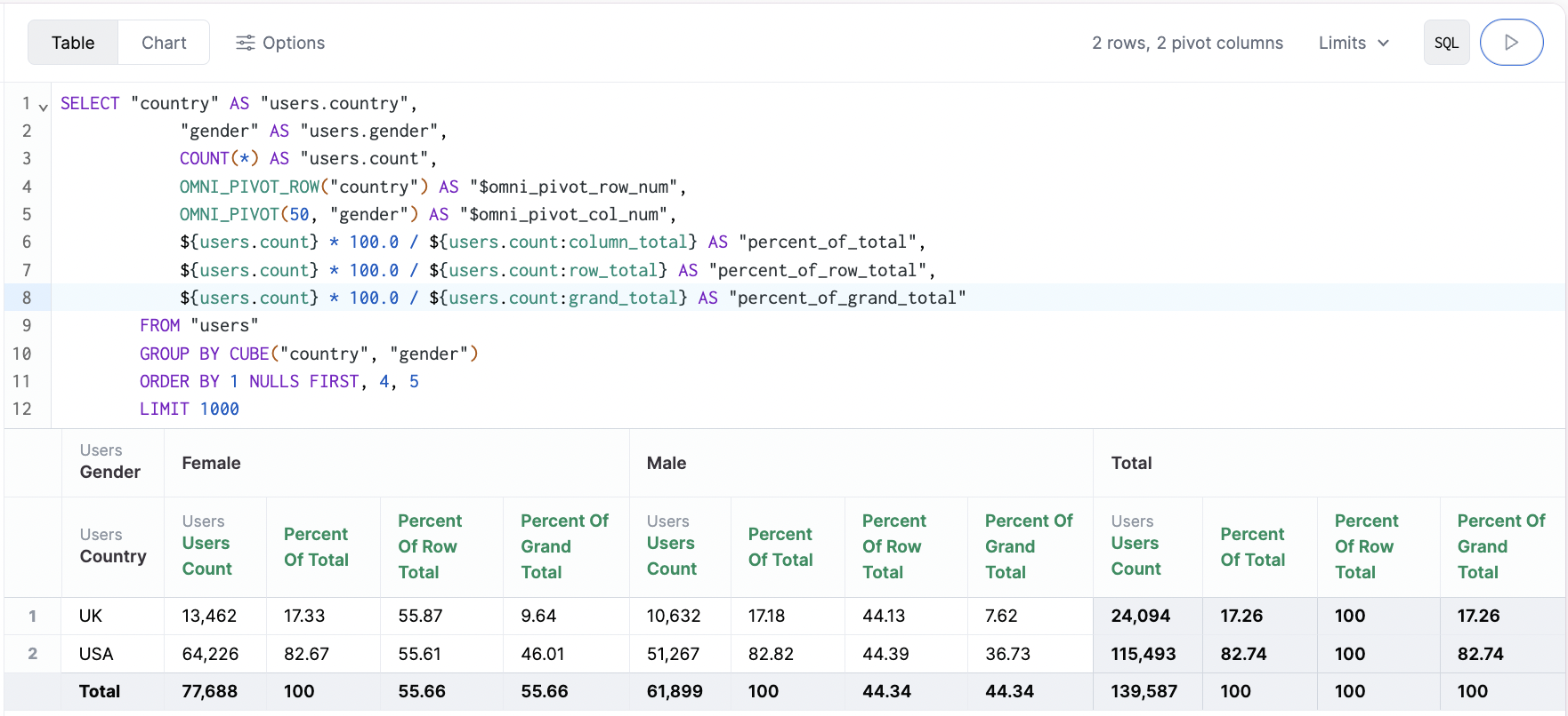
Using row and column totals can be effective for more complex calculations across rows or columns indepdently. These aggregates can be referenced in calculations when they are activated for queries (using the table options menu).
- Column total:
${users.count:column_total}
- Row total:
${users.count:row_total}
- Grand total (columns and rows, lower right):
${users.count:grand_total}
These can also be chained with other functions, for example a percent of row, ${users.count} * 100.0 / ${users.count:row_total}
.
Calculations can also be adjusted in the table options to rename or change formatting or decimals.
Internal Functions
There are some other functions you may see in the SQL that are not meant for end user use, but help make the SQL blocks easier to parse in normal usage.
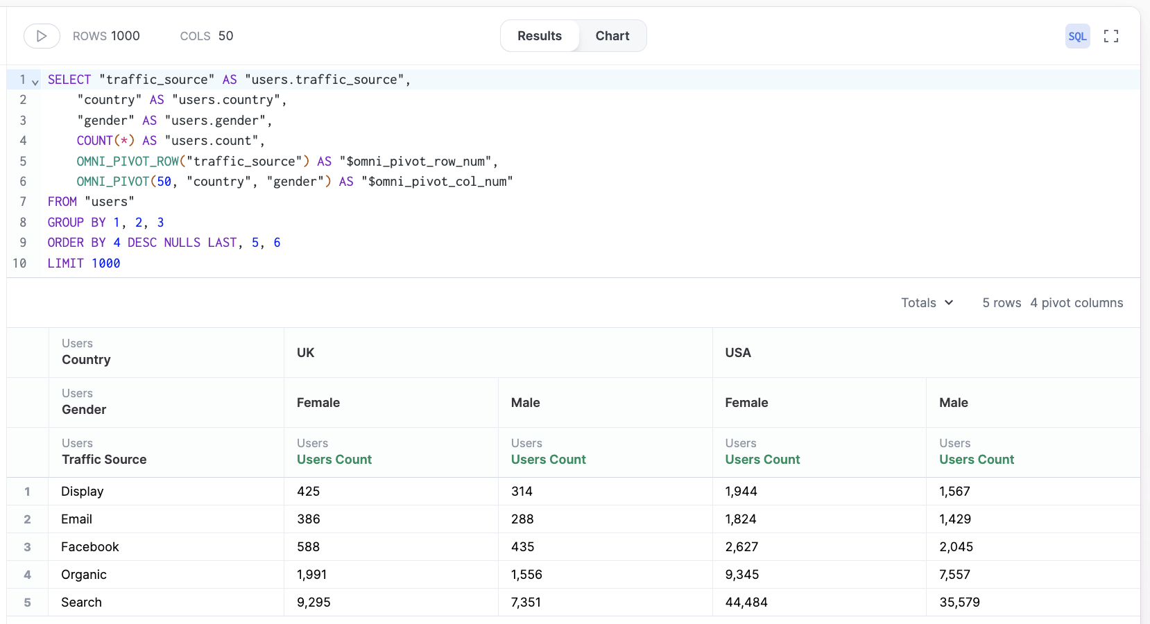
OMNI_PIVOT_ROW(dimensions), OMNI_PIVOT(column_limit, pivots)
- This pair of functions will structure the pivottable experience
OMNI_PIVOT_ROW
sets the query columns outside the pivotOMNI_PIVOT
set the query columns to be pivotted, along with a limit on columns- example:
Table Calculation Examples
Percent of Cohort - Gross Retention
Often for these calculations we need to look across a given cohort / row and understand the percentage of the group that was retained. To do calculations across pivots, we can simply use a given cell and then the context of the row or column. Below we show a few examples with ${users.count}
, and we can imagine they are grouped by ${users.sign_up[month]}
and ${users.months_since_sign_up}
OMNI_PIVOT_OFFSET()
offers some flexibility to use moving averages or lists. Here we divide each count by the max of the row, done using a column offset 100 columns back and 200 columns wide:
1.0 * ${users.count} / MAX(OMNI_OFFSET(${users.count}, 0, -100, 1, 200))
The alternative is using row_totals for simpler calculations:
1.0 ${users.count} / ${users.count:row_total}
Right now calculations cannot be pinned to the first column, so a window function would be required for % of first value, but this will open up soon.